NACA 2412 Open-Source CFD

Overview

Mississippi State’s Formula SAE team needs a repeatable 3D CFD workflow to complement its 2D analysis. In a guided NACA 2412 finite-wing benchmark, I prepared the Gmsh mesh, ran OpenFOAM, and inspected results in ParaView against historical wind-tunnel data. After 2,000 steady iterations, lift agreed closely with the approximate reference reading, while drag was about 50% higher. The case established a learning baseline; trailing-edge skewness and a pressure residual above the others require further investigation before the workflow can support reliable design decisions.

My Contribution

In this guided learning project, I carried out mesh preparation, OpenFOAM runs, and ParaView inspection using an assisted Gmsh script and step-by-step case-setup guidance. I examined mesh quality, residuals, forces, and comparison data, then prepared the findings for the team with assistance. My understanding of boundary conditions, discretization, k–ω SST, wall y+, and convergence grew substantially; I still need support when creating a new geometry script or choosing case parameters.

Engineering Approach

I chose Gmsh over a platform-generated mesh to gain direct control of the discretization. Unresolved mesh-import issues with SimScale led me to run the case locally in OpenFOAM instead. The finite aspect-ratio-6 wing was compared with the NACA reference at matched angle of attack and Reynolds number, with differences in experimental and modeling details retained as limitations.

Results & Current Status

The baseline reached 2,000 steady iterations: CL = 0.5255 and CD = 0.03584. Lift agrees closely with the approximate historical graph reading; drag is about 50% higher. Trailing-edge skewness and a pressure residual that settles above the other residuals motivate further investigation. Neither has been isolated as the cause of the drag discrepancy.

Gmsh → OpenFOAM → ParaView

1. Gmsh: Geometry & Mesh

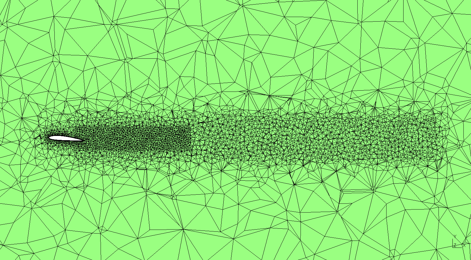
   The script imports the wing STEP geometry, builds 12 prism layers with a growth ratio of 1.15, and applies local refinement near the wing, wake, and tips. The final mesh contains 1,679,077 tetrahedra, 350,352 prisms, and 120 pyramids. It is exported as an ASCII MSH 2.2 file with metre coordinates.

2. OpenFOAM: Setup & Solution

   After conversion with gmshToFoam and mesh checks, the case runs steady incompressible RANS using SIMPLE, k–ω SST, and wall functions in OpenFOAM 12 through blueCFD-Core. Successful runs used six and then eight MPI processes on my Intel i7 laptop. I observed roughly 3–5 GB of RAM use; this is an approximate observation, not a recorded peak-memory benchmark. The final 1,500 iterations took about 86 minutes; all successful segments total 6,986 seconds. Timing excludes meshing, setup, post-processing, and an unsuccessful restart.

3. ParaView: Inspection & Communication

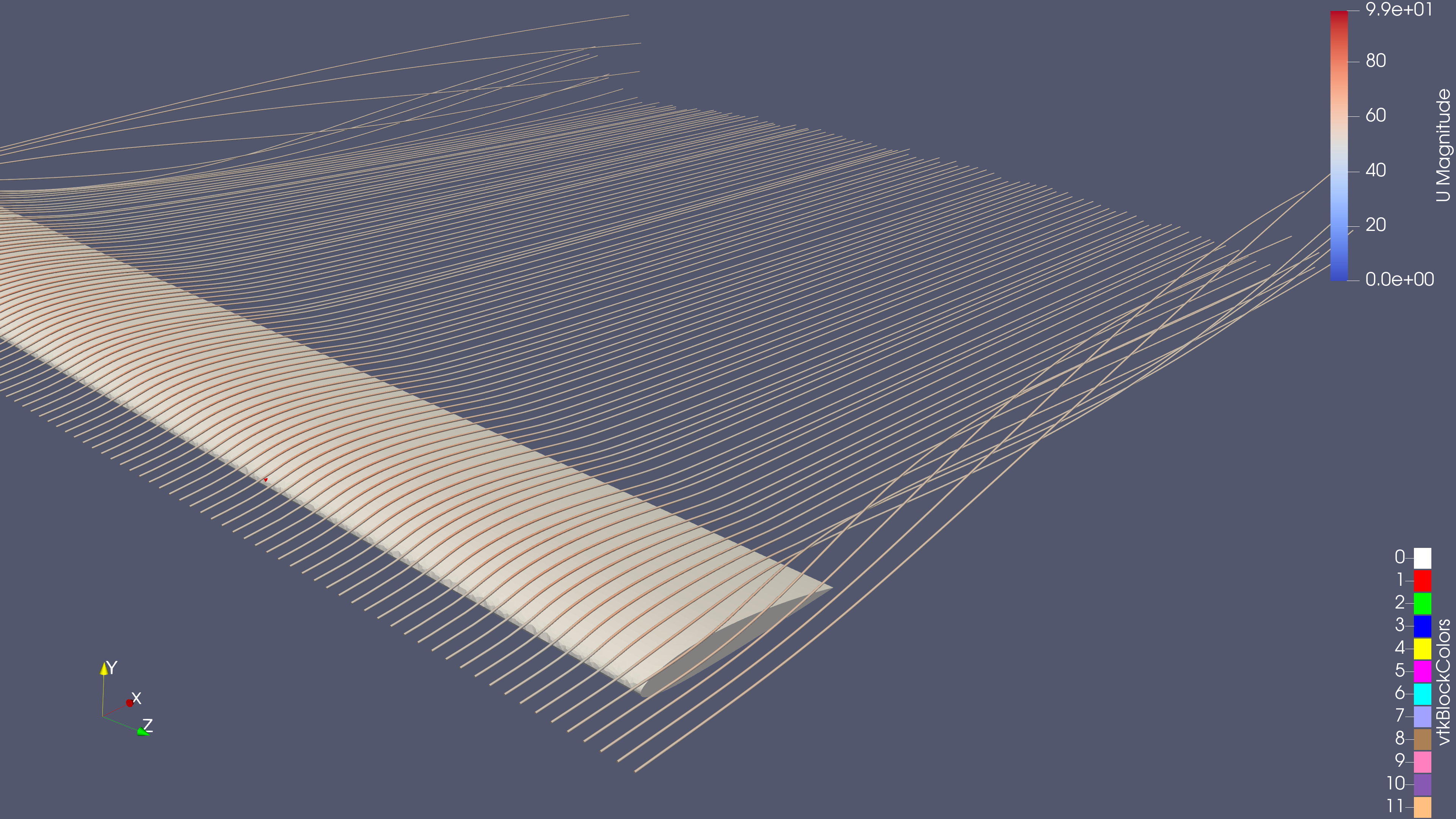
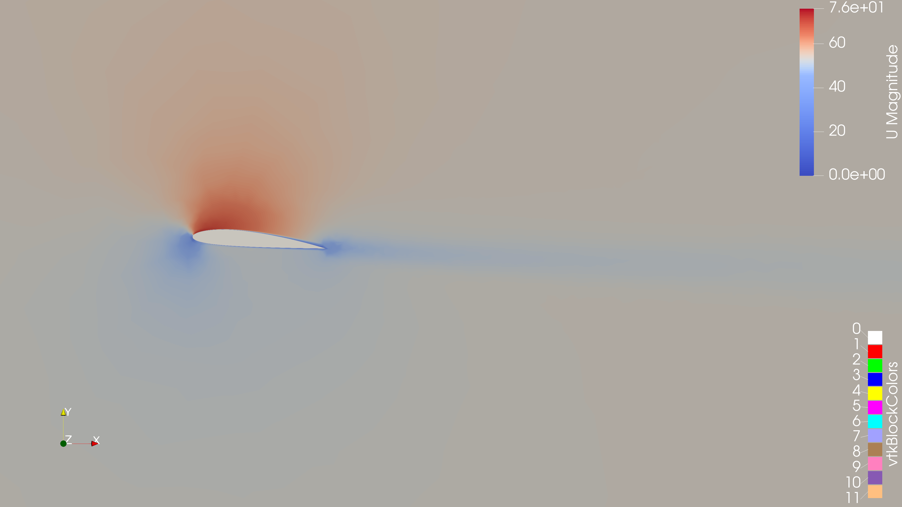
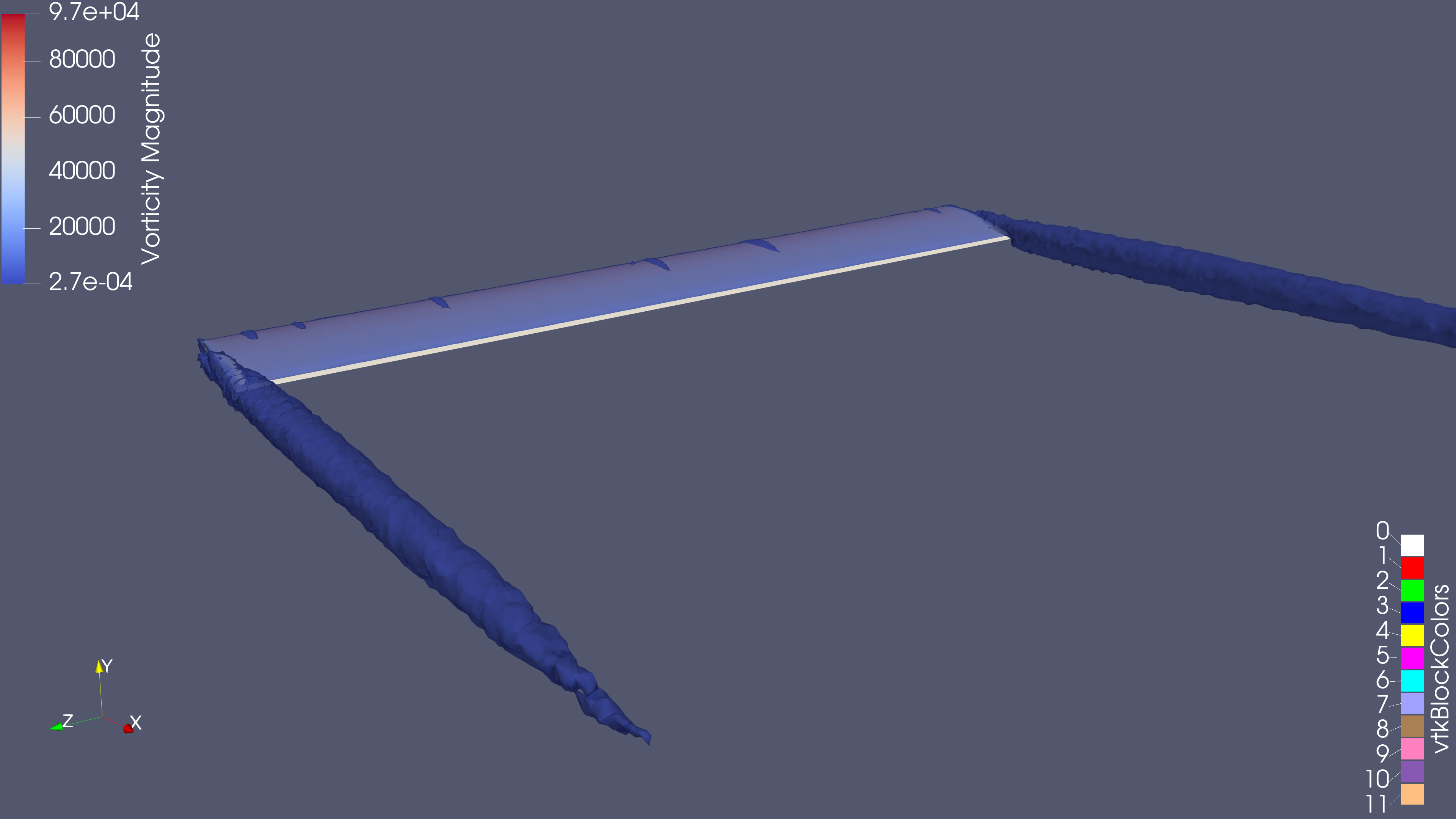
   I examined velocity slices, streamlines, wingtip vortex structures, wall y+, and mesh-quality markers. The saved state and team presentation capture this baseline for later comparison.

Benchmark Comparison

The simulated wing has a 0.9144 m chord, 5.4864 m full span, and aspect ratio 6. The case uses approximately 5° angle of attack, a freestream speed of 53.3136 m/s, and Reynolds number 3.25 million.

Lift falls within the visually estimated range. Drag is approximately 43–56% higher than that range, or about 50% high. The ranges are approximate graph readings, not experimental error bars. Historical turbulence, transition, and trailing-edge details are not an exact match to this case, and agreement at one operating point does not establish validation across other conditions.

Reference: NACA Report 460, Figure 18 . The finite-aspect-ratio curves are used for this comparison; the infinite-aspect-ratio panel is a different reference.

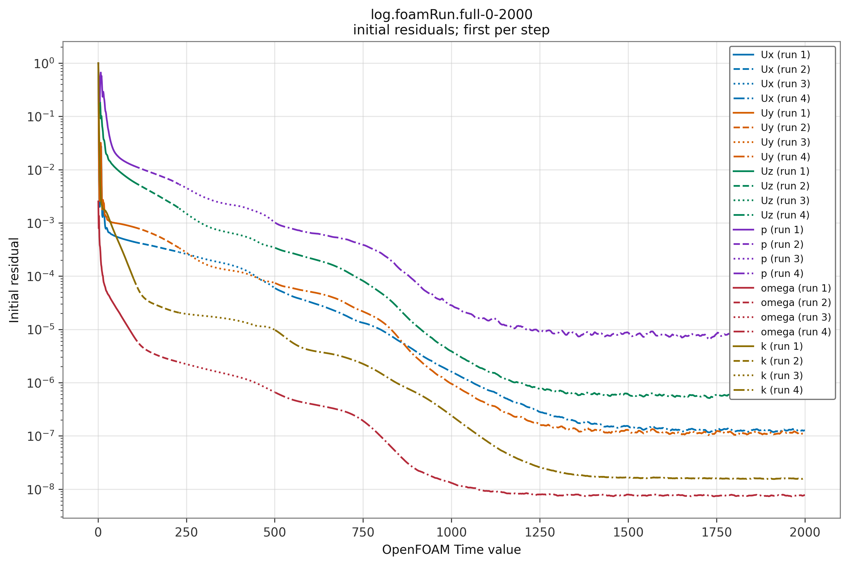
At iteration 2000, initial pressure residual was about 7.59 × 10⁻⁶ and the largest velocity-component residual was about 5.44 × 10⁻⁷. The pressure residual lags behind the velocity and turbulence residuals and settles at a higher level. Incomplete pressure convergence could contribute to the drag overestimate, so the pressure residual and drag need further investigation and research. Residual magnitudes from different equations are not directly comparable measures of physical error, and this run has not established a causal relationship. Force coefficients were nearly unchanged late in the run. This numerical settling is useful evidence, but it does not remove mesh errors or establish physical accuracy.

Mesh Quality & Limitations

checkMesh failed two checks: 2,136 highly skewed faces (maximum skewness 16.1669) and two unused points. It also reported 42 faces above 70° non-orthogonality, with a maximum of 77.7987°. The flagged faces concentrate along the trailing edge, where the prism layers visibly distort.

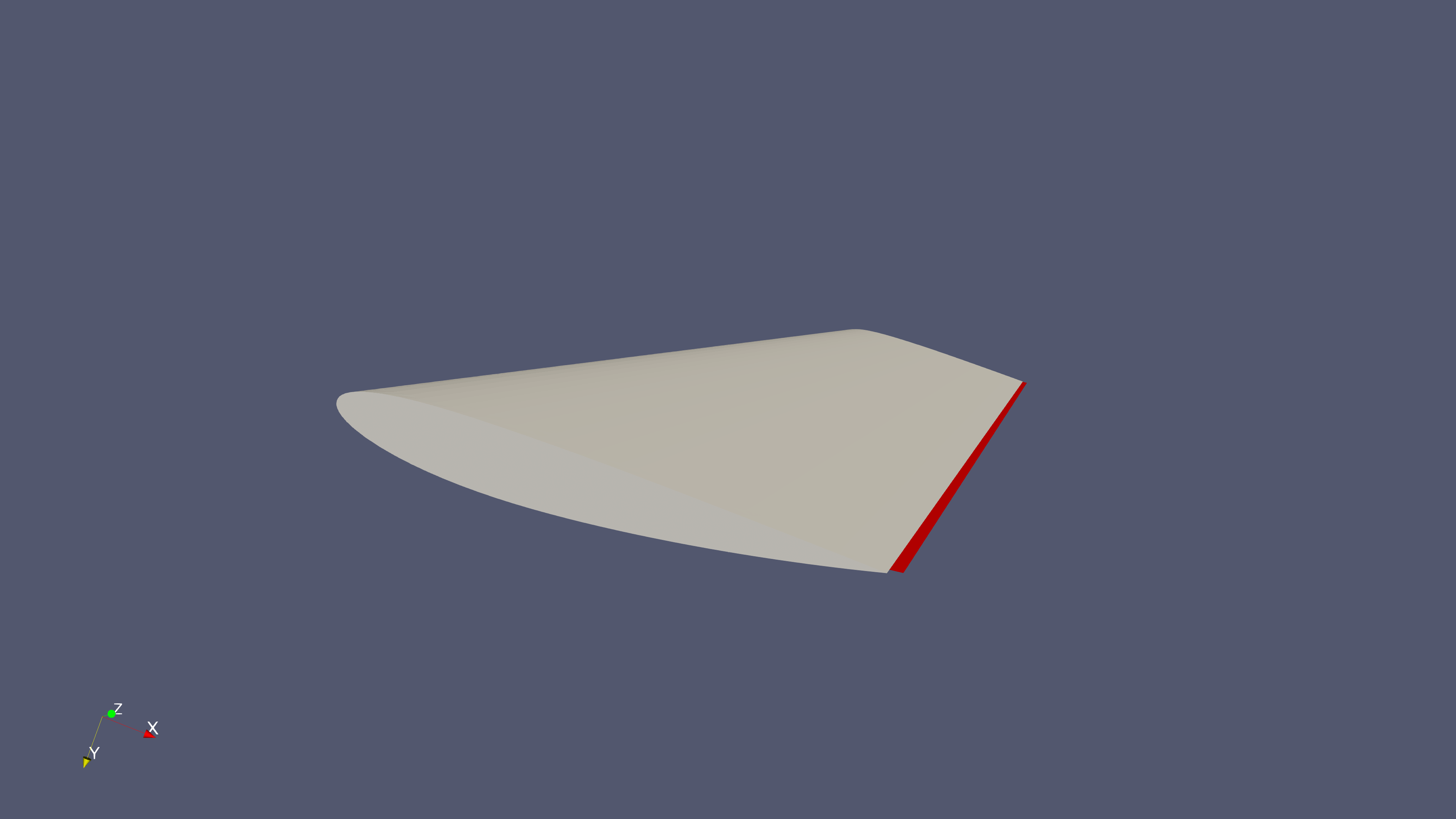
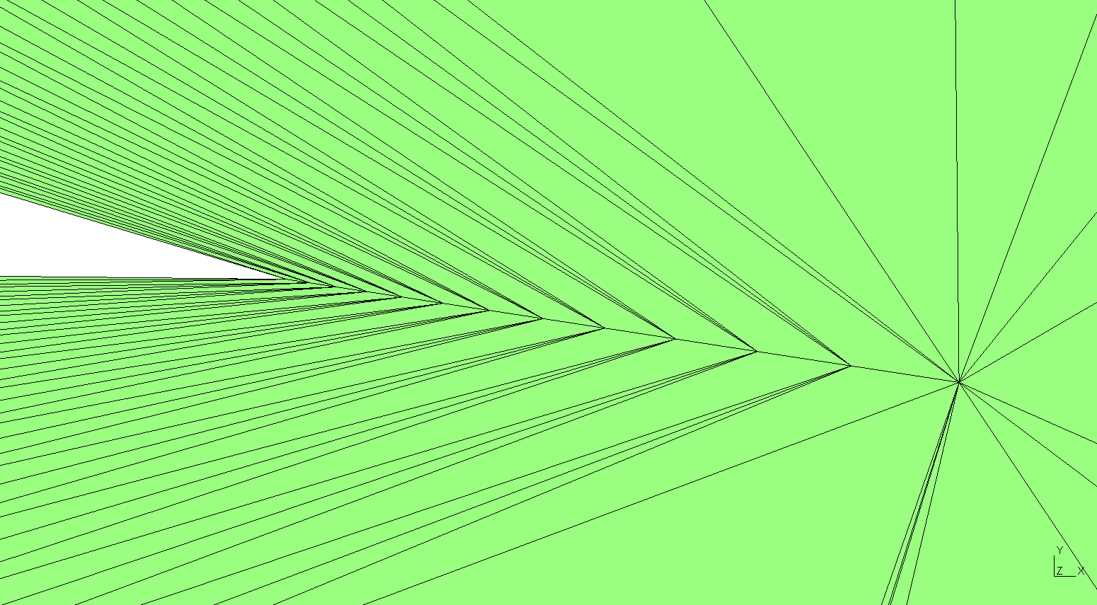
The mesh issue is a plausible contributor to the drag discrepancy, but its contribution has not been isolated. A controlled remesh and rerun is needed to separate mesh effects from turbulence/transition assumptions, discretization, geometry details, and differences from the historical experiment.

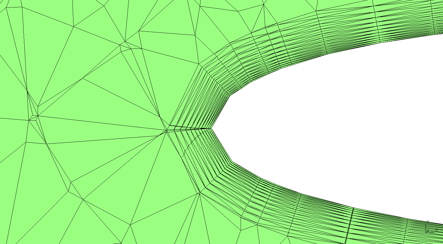
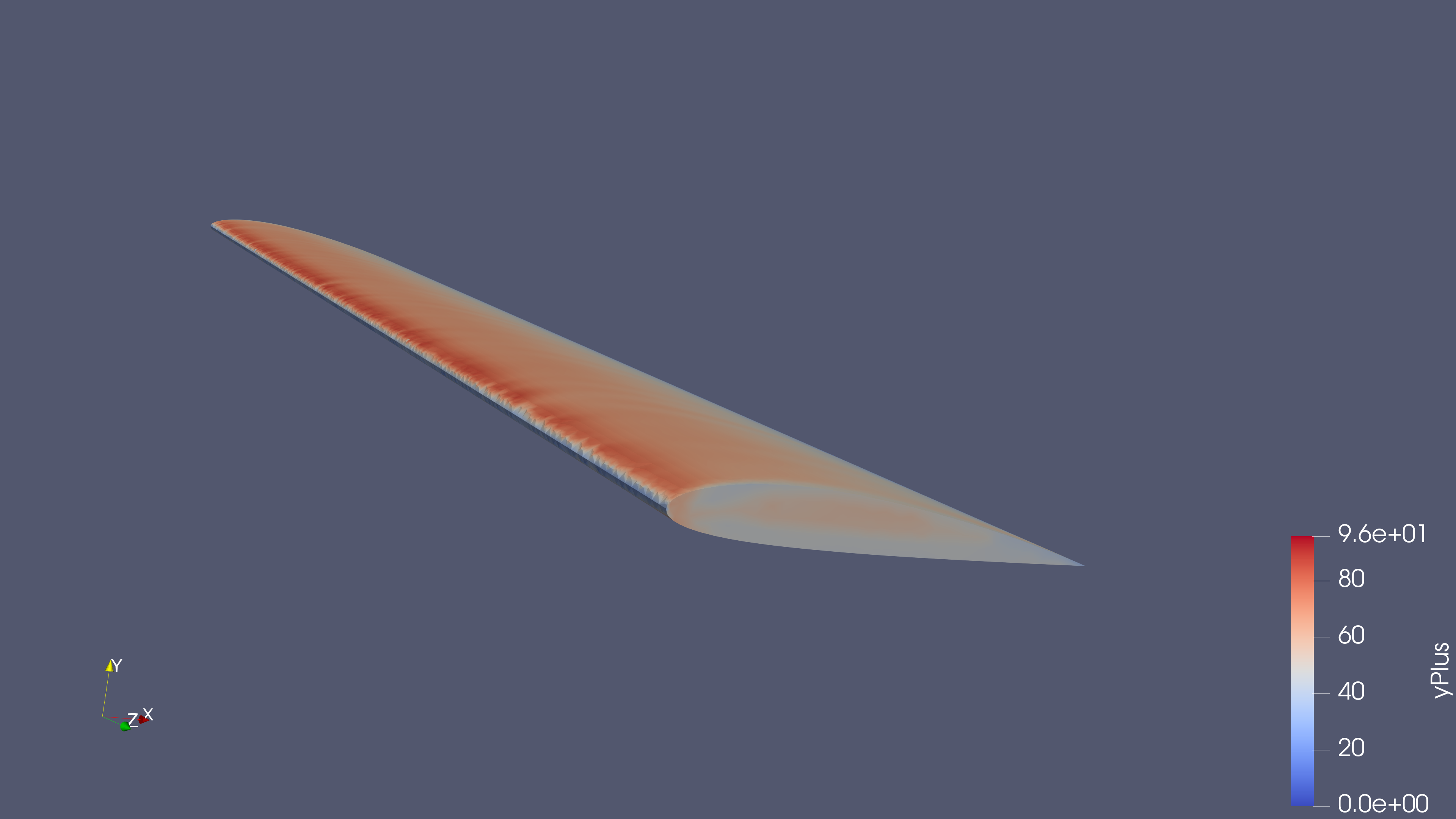
The wall y+ distribution should be reviewed alongside the chosen wall-function treatment. The final run includes the small defaultFaces patch in force accounting; patch completeness and boundary classification remain part of the mesh review.

Next Steps

1. Repair the trailing edge. Revisit the geometry and layer extrusion, remove unused points, and inspect all boundary patches. Run checkMesh again before solving.
2. Repeat the same operating point. Hold solver settings, reference area, force axes, and flow conditions constant to measure what changes after the mesh repair.
3. Investigate pressure convergence and drag. Research pressure-solver tolerances, pressure–velocity coupling, and discretization choices; continue controlled runs and track pressure and viscous drag separately. Compare changes in the pressure residual with force stability to test whether incomplete pressure convergence contributes to the drag overestimate.
4. Check sensitivity and correlation. Compare at least three mesh levels, inspect y+, track forces as well as residuals, and run an angle-of-attack sweep against the historical reference.
5. Apply the process to an isolated FSAE wing. Use the benchmark lessons to set up a component study before progressing toward interacting aeropackage or full-car cases.
6. Build a repeatable team handoff. Keep CAD, mesh scripts, solver inputs, run logs, and ParaView states together, and continue learning the setup decisions so I can execute the workflow more independently.

Supporting Files & Model

Download the team presentation, original wing geometry, or documented setup and analysis records.

• 3D visualization ↓ (download GLB)GLB · 527 KB
• Wing CAD geometry ↓ (download STEP)STEP · 37 KB
• Team presentation ↓ (download PPTX)PPTX · 4.7 MB
• Rebuild & analysis package ↓ (download ZIP)ZIP · 888 KB
• Residual history ↓ (download CSV)CSV · 73 KB

The ZIP includes STEP geometry, the commented Gmsh script, historical OpenFOAM inputs and analysis, and tested rebuild/ParaView helpers. Follow the README to generate the mesh, set wall patches, solve from iteration zero, and open your results in ParaView. A fresh two-iteration startup test passed; the full 2,000-iteration study was not rerun. The known skew-face defects remain. Large generated meshes and solved fields are excluded to keep the download small. The standalone STEP and the geometry inside the ZIP are identical.

Browse the Model Library →